Searches through the vector of lag orders to find the best AR model which
has lowest AIC, AICc or BIC value. It is implemented using OLS, and behaves
comparably to stats::ar.ols().
AR(formula, ic = c("aicc", "aic", "bic"), ...)Arguments
Value
A model specification.
Details
Exogenous regressors and common_xregs can be specified in the model
formula.
Specials
pdq
The order special is used to specify the lag order for the auto-regression.
p | The order of the auto-regressive (AR) terms. If multiple values are provided, the one which minimises ic will be chosen. |
fixed | A named list of fixed parameters for coefficients. The names identify the coefficient, beginning with ar, and then followed by the lag order. For example, fixed = list(ar1 = 0.3, ar3 = 0). |
xreg
Exogenous regressors can be included in an AR model without explicitly using the xreg() special. Common exogenous regressor specials as specified in common_xregs can also be used. These regressors are handled using stats::model.frame(), and so interactions and other functionality behaves similarly to stats::lm().
The inclusion of a constant in the model follows the similar rules to stats::lm(), where including 1 will add a constant and 0 or -1 will remove the constant. If left out, the inclusion of a constant will be determined by minimising ic.
xreg(..., fixed = list())... | Bare expressions for the exogenous regressors (such as log(x)) |
fixed | A named list of fixed parameters for coefficients. The names identify the coefficient, and should match the name of the regressor. For example, fixed = list(constant = 20). |
Examples
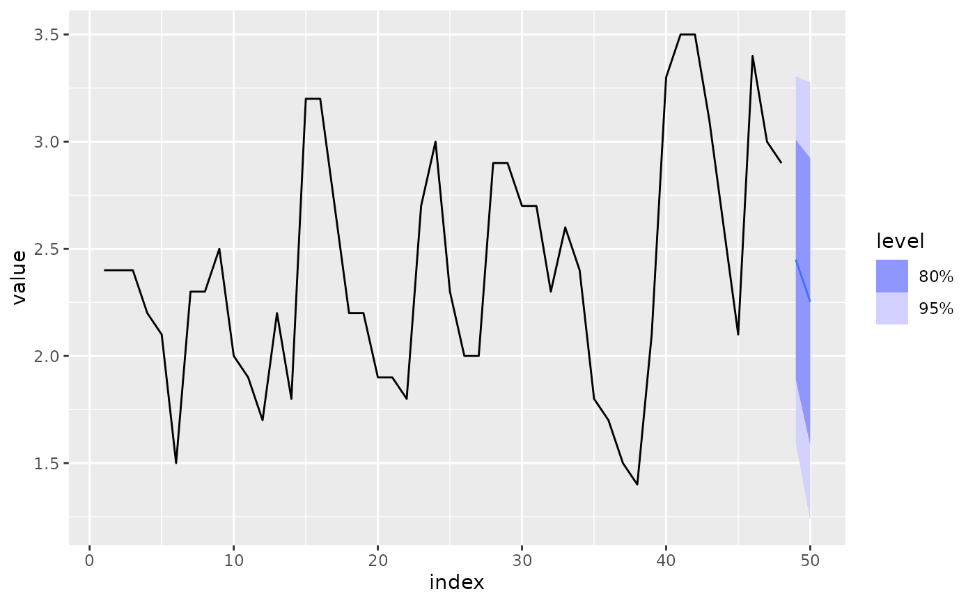
luteinizing_hormones <- as_tsibble(lh)
fit <- luteinizing_hormones %>%
  model(AR(value ~ order(3)))

report(fit)
#> Series: value
#> Model: AR(3) w/ mean
#>
#> Coefficients:
#>   constant     ar1      ar2      ar3
#>     1.5375  0.6578  -0.0658  -0.2348
#>
#> sigma^2 estimated as 0.1905
#> AIC = -14.48	AICc = -13.55	BIC = -7

fit %>%
  forecast() %>%
  autoplot(luteinizing_hormones)
