The fable package provides some commonly used univariate and multivariate time series forecasting models which can be used with tidy temporal data in the tsibble format. These models are used within a consistent and tidy modelling framework, allowing several models to be estimated, compared, combined, forecasted and otherwise worked with across many time series.
Suppose we wanted to forecast the number of domestic travellers to
Melbourne, Australia. In the tsibble::tourism data set,
this can be further broken down into 4 reasons of travel: “business”,
“holiday”, “visiting friends and relatives” and “other reasons”. The
first observation from each series are shown below.
tourism_melb <- tourism %>%
  filter(Region == "Melbourne")
tourism_melb %>%
  group_by(Purpose) %>%
  slice(1)
#> # A tsibble: 4 x 5 [1Q]
#> # Key:       Region, State, Purpose [4]
#> # Groups:    Purpose [4]
#>   Quarter Region    State    Purpose  Trips
#>     <qtr> <chr>     <chr>    <chr>    <dbl>
#> 1 1998 Q1 Melbourne Victoria Business 405.
#> 2 1998 Q1 Melbourne Victoria Holiday  428.
#> 3 1998 Q1 Melbourne Victoria Other     79.9
#> 4 1998 Q1 Melbourne Victoria Visiting 666.
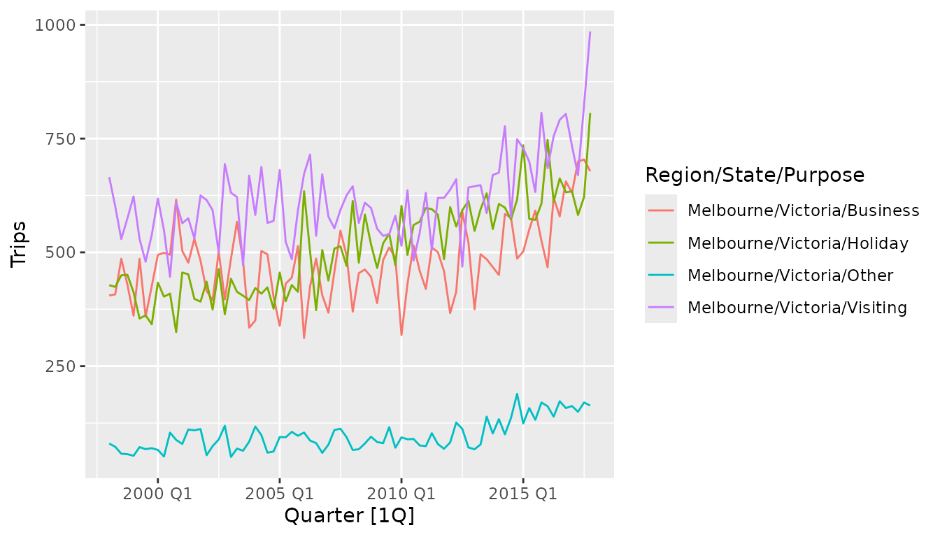
The variable that we’d like to estimate is the number of overnight
trips (in thousands) represented by the Trips variable. A
plot of the data reveals that some trends and weak seasonality are
apparent.

Two widely used models available in this package are ETS and ARIMA.
These models are specified using a compact formula representation (much
like cross-sectional linear models using lm()). The
response variable (Trips) and any transformations are
included on the left, while the model specification is on the right of
the formula. When a model is not fully specified (or if the formula’s
right side is missing completely), the unspecified components will be
chosen automatically.
Suppose we think that the ETS model must have an additive trend, and
want the other elements to be chosen automatically. This model would be
specified using ETS(Trips ~ trend("A")). Similarly, a
completely automatic ARIMA model (much like auto.arima()
from the forecast package) can be specified using
ARIMA(Trips). The model() function is used to
estimate these model specifications on a particular dataset, and will
return a “mable” (model table).
fit <- tourism_melb %>%
  model(
    ets = ETS(Trips ~ trend("A")),
    arima = ARIMA(Trips)
  )
fit
#> # A mable: 4 x 5
#> # Key:     Region, State, Purpose [4]
#>   Region    State    Purpose           ets                             arima
#>   <chr>     <chr>    <chr>         <model>                           <model>
#> 1 Melbourne Victoria Business <ETS(A,A,A)> <ARIMA(0,1,2)(1,0,1)[4] w/ drift>
#> 2 Melbourne Victoria Holiday  <ETS(M,A,A)>           <ARIMA(0,1,1) w/ drift>
#> 3 Melbourne Victoria Other    <ETS(A,A,N)>           <ARIMA(0,1,1) w/ drift>
#> 4 Melbourne Victoria Visiting <ETS(M,A,A)>          <ARIMA(0,1,1)(1,0,2)[4]>
A mable contains a row for each time series (uniquely identified by the key variables), and a column for each model specification. A model is contained within the cells of each model column. In the example above we can see that the all four ETS models have an additive trend, and the error and seasonality have been chosen automatically. Similarly, the ARIMA model varies between time series as it has been automatically selected.
The coef() or tidy() function is used to
extract the coefficients from the models. It’s possible to use
select() and other verbs to focus on the coefficients from
a particular model.
fit %>%
  select(Region, State, Purpose, arima) %>%
  coef()
#> # A tibble: 13 × 9
#>    Region    State    Purpose .model term  estimate std.error statistic  p.value
#>    <chr>     <chr>    <chr>   <chr>  <chr>    <dbl>     <dbl>     <dbl>    <dbl>
#>  1 Melbourne Victoria Busine… arima  ma1     -0.555    0.130     -4.28  5.29e- 5
#>  2 Melbourne Victoria Busine… arima  ma2     -0.233    0.129     -1.81  7.47e- 2
#>  3 Melbourne Victoria Busine… arima  sar1     0.946    0.0634    14.9   1.08e-24
#>  4 Melbourne Victoria Busine… arima  sma1    -0.772    0.145     -5.34  8.81e- 7
#>  5 Melbourne Victoria Busine… arima  cons…    0.192    0.213      0.903 3.69e- 1
#>  6 Melbourne Victoria Holiday arima  ma1     -0.931    0.0851   -10.9   1.77e-17
#>  7 Melbourne Victoria Holiday arima  cons…    3.65     0.571      6.39  1.06e- 8
#>  8 Melbourne Victoria Other   arima  ma1     -0.750    0.0708   -10.6   8.19e-17
#>  9 Melbourne Victoria Other   arima  cons…    1.24     0.640      1.93  5.70e- 2
#> 10 Melbourne Victoria Visiti… arima  ma1     -0.838    0.0652   -12.8   5.03e-21
#> 11 Melbourne Victoria Visiti… arima  sar1     0.659    0.193      3.41  1.03e- 3
#> 12 Melbourne Victoria Visiti… arima  sma1    -0.402    0.206     -1.95  5.47e- 2
#> 13 Melbourne Victoria Visiti… arima  sma2     0.322    0.143      2.26  2.68e- 2
The glance() function provides a one-row summary of each
model, and commonly includes descriptions of the model’s fit such as the
residual variance and information criteria. Be wary though, as
information criteria (AIC, AICc, BIC) are only comparable between the
same model class and only if those models share the same response (after
transformations and differencing).
fit %>%
  glance()
#> # A tibble: 8 × 14
#>   Region    State   Purpose .model  sigma2 log_lik   AIC  AICc   BIC   MSE  AMSE
#>   <chr>     <chr>   <chr>   <chr>    <dbl>   <dbl> <dbl> <dbl> <dbl> <dbl> <dbl>
#> 1 Melbourne Victor… Busine… ets    3.53e+3   -498. 1014. 1016. 1035. 3180. 3520.
#> 2 Melbourne Victor… Busine… arima  3.67e+3   -435.  882.  883.  896.   NA    NA
#> 3 Melbourne Victor… Holiday ets    1.10e-2   -487.  992.  994. 1013. 2548. 2574.
#> 4 Melbourne Victor… Holiday arima  3.07e+3   -429.  864.  865.  872.   NA    NA
#> 5 Melbourne Victor… Other   ets    4.97e+2   -422.  853.  854.  865.  472.  512.
#> 6 Melbourne Victor… Other   arima  4.89e+2   -356.  718.  719.  725.   NA    NA
#> 7 Melbourne Victor… Visiti… ets    1.09e-2   -503. 1024. 1026. 1045. 3714. 3860.
#> 8 Melbourne Victor… Visiti… arima  4.24e+3   -442.  893.  894.  905.   NA    NA
#> # ℹ 3 more variables: MAE <dbl>, ar_roots <list>, ma_roots <list>
If you’re working with a single model (or want to look at one model
in particular), the report() function gives a familiar and
nicely formatted model-specific display.
fit %>%
  filter(Purpose == "Holiday") %>%
  select(ets) %>%
  report()
#> Series: Trips
#> Model: ETS(M,A,A)
#>   Smoothing parameters:
#>     alpha = 0.03084501
#>     beta  = 0.03084499
#>     gamma = 0.0001000967
#>
#>   Initial states:
#>      l[0]      b[0]     s[0]    s[-1]     s[-2]    s[-3]
#>  424.0777 -2.535481 -26.7441 4.256618 -10.10668 32.59417
#>
#>   sigma^2:  0.011
#>
#>       AIC      AICc       BIC
#>  991.7305  994.3020 1013.1688
The fitted values and residuals from a model can obtained using
fitted() and residuals() respectively.
Additionally, the augment() function may be more
convenient, which provides the original data along with both fitted
values and their residuals.
fit %>%
  augment()
#> # A tsibble: 640 x 9 [1Q]
#> # Key:       Region, State, Purpose, .model [8]
#>    Region    State    Purpose  .model Quarter Trips .fitted  .resid  .innov
#>    <chr>     <chr>    <chr>    <chr>    <qtr> <dbl>   <dbl>   <dbl>   <dbl>
#>  1 Melbourne Victoria Business ets    1998 Q1  405.    396.    9.54    9.54
#>  2 Melbourne Victoria Business ets    1998 Q2  408.    483.  -75.1   -75.1
#>  3 Melbourne Victoria Business ets    1998 Q3  486.    487.   -1.13   -1.13
#>  4 Melbourne Victoria Business ets    1998 Q4  429.    454.  -25.2   -25.2
#>  5 Melbourne Victoria Business ets    1999 Q1  361.    391.  -30.3   -30.3
#>  6 Melbourne Victoria Business ets    1999 Q2  486.    466.   19.9    19.9
#>  7 Melbourne Victoria Business ets    1999 Q3  359.    492. -133.   -133.
#>  8 Melbourne Victoria Business ets    1999 Q4  426.    424.    1.49    1.49
#>  9 Melbourne Victoria Business ets    2000 Q1  495.    364.  130.    130.
#> 10 Melbourne Victoria Business ets    2000 Q2  499.    477.   22.0    22.0
#> # ℹ 630 more rows
To compare how well the models fit the data, we can consider some common accuracy measures. It seems that on the training set the ETS model out-performs ARIMA for the series where travellers are on holiday, business, and visiting friends and relatives. The Evaluating modelling accuracy chapter from the Forecasting: Principles and Practices (3rd Ed.) textbook provides more detail in how modelling and forecasting accuracy is evaluated.
fit %>%
  accuracy() %>%
  arrange(MASE)
#> # A tibble: 8 × 13
#>   Region  State Purpose .model .type     ME  RMSE   MAE    MPE  MAPE  MASE RMSSE
#>   <chr>   <chr> <chr>   <chr>  <chr>  <dbl> <dbl> <dbl>  <dbl> <dbl> <dbl> <dbl>
#> 1 Melbou… Vict… Holiday ets    Trai…  4.67   50.5  37.2  0.217  7.29 0.675 0.697
#> 2 Melbou… Vict… Busine… ets    Trai…  3.31   56.4  42.9 -0.753  9.31 0.691 0.740
#> 3 Melbou… Vict… Busine… arima  Trai…  2.54   58.2  46.0 -1.17  10.1  0.741 0.765
#> 4 Melbou… Vict… Holiday arima  Trai… -4.64   54.3  41.4 -2.44   8.46 0.752 0.751
#> 5 Melbou… Vict… Other   arima  Trai… -0.344  21.7  17.0 -6.16  19.5  0.763 0.772
#> 6 Melbou… Vict… Other   ets    Trai… -0.142  21.7  17.0 -5.97  19.6  0.767 0.773
#> 7 Melbou… Vict… Visiti… ets    Trai…  8.17   60.9  51.4  0.433  8.28 0.819 0.782
#> 8 Melbou… Vict… Visiti… arima  Trai…  6.89   63.1  51.7  0.106  8.44 0.825 0.809
#> # ℹ 1 more variable: ACF1 <dbl>
Forecasts from these models can be produced directly as our specified models do not require any additional data.
fc <- fit %>%
  forecast(h = "5 years")
fc
#> # A fable: 160 x 7 [1Q]
#> # Key:     Region, State, Purpose, .model [8]
#>    Region    State    Purpose  .model Quarter
#>    <chr>     <chr>    <chr>    <chr>    <qtr>
#>  1 Melbourne Victoria Business ets    2018 Q1
#>  2 Melbourne Victoria Business ets    2018 Q2
#>  3 Melbourne Victoria Business ets    2018 Q3
#>  4 Melbourne Victoria Business ets    2018 Q4
#>  5 Melbourne Victoria Business ets    2019 Q1
#>  6 Melbourne Victoria Business ets    2019 Q2
#>  7 Melbourne Victoria Business ets    2019 Q3
#>  8 Melbourne Victoria Business ets    2019 Q4
#>  9 Melbourne Victoria Business ets    2020 Q1
#> 10 Melbourne Victoria Business ets    2020 Q2
#> # ℹ 150 more rows
#> # ℹ 2 more variables: Trips <dist>, .mean <dbl>
The resulting forecasts are contained in a “fable” (forecast table),
and both point forecasts and forecast distributions are available in the
table for the next five years. Confidence intervals can be extracted
from the distribution using the hilo() function.
The hilo() function can also be used on fable objects,
which allows you to extract multiple intervals at once.
fc %>%
  hilo(level = c(80, 95))
#> # A tsibble: 160 x 9 [1Q]
#> # Key:       Region, State, Purpose, .model [8]
#>    Region    State    Purpose  .model Quarter
#>    <chr>     <chr>    <chr>    <chr>    <qtr>
#>  1 Melbourne Victoria Business ets    2018 Q1
#>  2 Melbourne Victoria Business ets    2018 Q2
#>  3 Melbourne Victoria Business ets    2018 Q3
#>  4 Melbourne Victoria Business ets    2018 Q4
#>  5 Melbourne Victoria Business ets    2019 Q1
#>  6 Melbourne Victoria Business ets    2019 Q2
#>  7 Melbourne Victoria Business ets    2019 Q3
#>  8 Melbourne Victoria Business ets    2019 Q4
#>  9 Melbourne Victoria Business ets    2020 Q1
#> 10 Melbourne Victoria Business ets    2020 Q2
#> # ℹ 150 more rows
#> # ℹ 4 more variables: Trips <dist>, .mean <dbl>, `80%` <hilo>, `95%` <hilo>
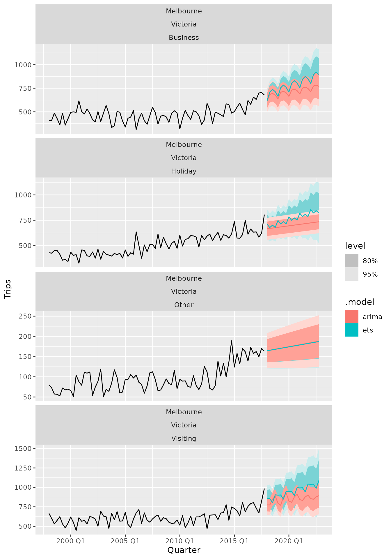
You can also see a plot of the forecasts using
autoplot(). To see the historical data along with the
forecasts you can provide it as the first argument to the function.

More model methods may be supported by particular models, including
the ability to refit() the model to new data,
stream() in new data to extend the fit,
generate() simulated paths from a model,
interpolate() missing values, extract
components() from the fitted model, and display the model’s
equation().
More information about modelling time series and using the fable package can be found in Forecasting: Principles and Practices (3rd Ed.) and in the pkgdown site.