Searches through the vector of lag orders to find the best VAR model which has lowest AIC, AICc or BIC value. It is implemented using OLS per equation.
VAR(formula, ic = c("aicc", "aic", "bic"), ...)Arguments
Value
A model specification.
Details
Exogenous regressors and common_xregs can be specified in the model
formula.
Specials
AR
The AR special is used to specify the lag order for the auto-regression.
AR(p = 0:5)p | The order of the auto-regressive (AR) terms. If multiple values are provided, the one which minimises ic will be chosen. |
xreg
Exogenous regressors can be included in an VAR model without explicitly using the xreg() special. Common exogenous regressor specials as specified in common_xregs can also be used. These regressors are handled using stats::model.frame(), and so interactions and other functionality behaves similarly to stats::lm().
The inclusion of a constant in the model follows the similar rules to stats::lm(), where including 1 will add a constant and 0 or -1 will remove the constant. If left out, the inclusion of a constant will be determined by minimising ic.
xreg(...)... | Bare expressions for the exogenous regressors (such as log(x)) |
Examples
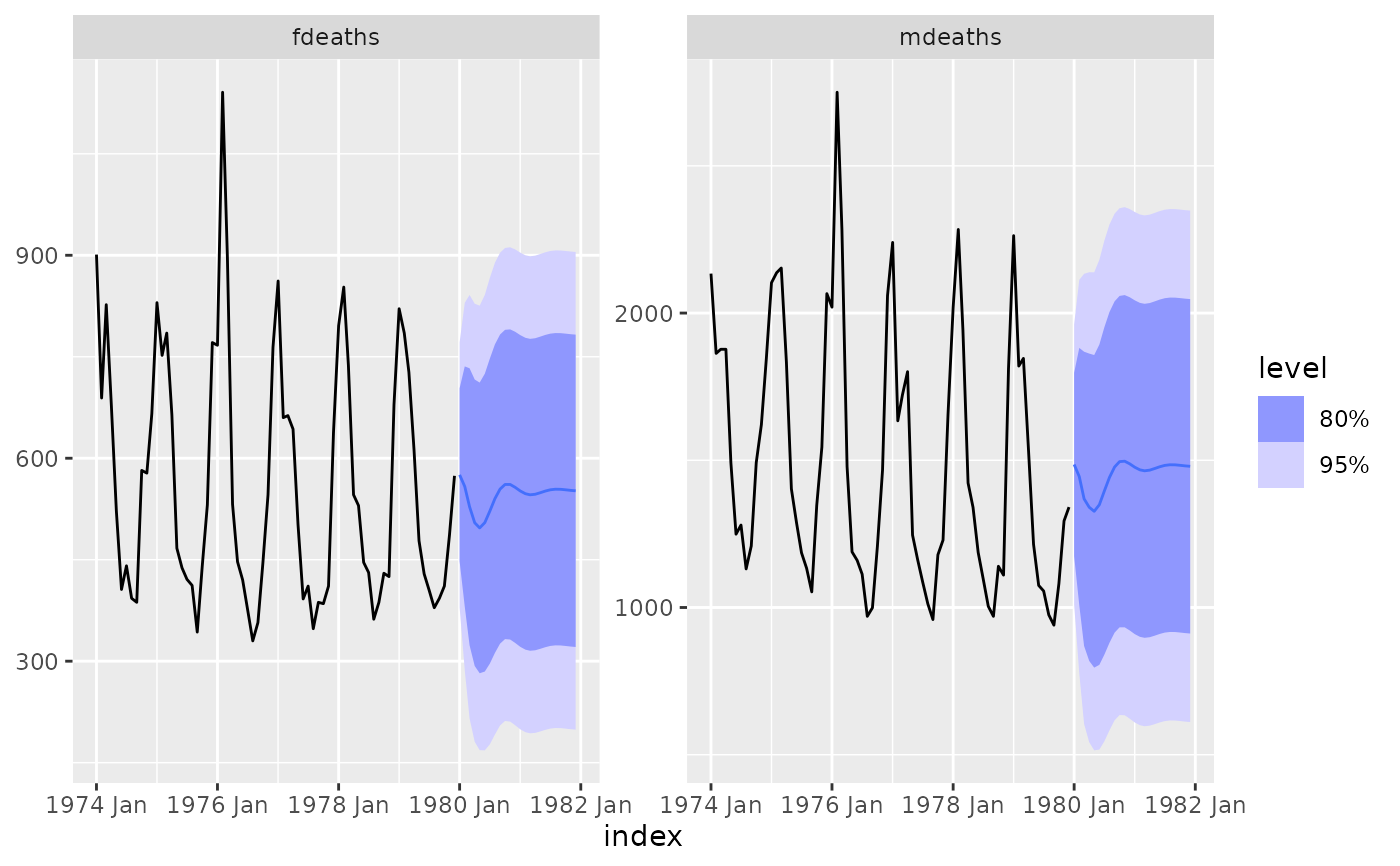
lung_deaths <- cbind(mdeaths, fdeaths) %>%
  as_tsibble(pivot_longer = FALSE)

fit <- lung_deaths %>%
  model(VAR(vars(mdeaths, fdeaths) ~ AR(3)))

report(fit)
#> Series: mdeaths, fdeaths
#> Model: VAR(3) w/ mean
#>
#> Coefficients for mdeaths:
#>       lag(mdeaths,1)  lag(fdeaths,1)  lag(mdeaths,2)  lag(fdeaths,2)
#>               0.6675          0.8074          0.3677         -1.4540
#> s.e.          0.3550          0.8347          0.3525          0.8088
#>       lag(mdeaths,3)  lag(fdeaths,3)  constant
#>               0.2606         -1.1214  538.7817
#> s.e.          0.3424          0.8143  137.1047
#>
#> Coefficients for fdeaths:
#>       lag(mdeaths,1)  lag(fdeaths,1)  lag(mdeaths,2)  lag(fdeaths,2)
#>               0.2138          0.4563          0.0937         -0.3984
#> s.e.          0.1460          0.3434          0.1450          0.3328
#>       lag(mdeaths,3)  lag(fdeaths,3)  constant
#>               0.0250          -0.315  202.0027
#> s.e.          0.1409           0.335   56.4065
#>
#> Residual covariance matrix:
#>          mdeaths  fdeaths
#> mdeaths 58985.95 22747.94
#> fdeaths 22747.94  9983.95
#>
#> log likelihood = -812.35
#> AIC = 1660.69	AICc = 1674.37	BIC = 1700.9

fit %>%
  forecast() %>%
  autoplot(lung_deaths)