Estimate a VECM model

Searches through the vector of lag orders to find the best VECM model which has lowest AIC, AICc or BIC value. The model is estimated using the Johansen procedure (maximum likelihood).

VECM(formula, ic = c("aicc", "aic", "bic"), r = 1L, ...)

Arguments

formula

Model specification (see "Specials" section).

ic

The information criterion used in selecting the model.

r

The number of cointegrating relationships

...

Further arguments for arima

Value

A model specification.

Details

Exogenous regressors and common_xregs can be specified in the model formula.

Specials

AR

The AR special is used to specify the lag order for the auto-regression.

AR(p = 0:5)

p	The order of the auto-regressive (AR) terms. If multiple values are provided, the one which minimises ic will be chosen.

xreg

Exogenous regressors can be included in an VECM model without explicitly using the xreg() special. Common exogenous regressor specials as specified in common_xregs can also be used. These regressors are handled using stats::model.frame(), and so interactions and other functionality behaves similarly to stats::lm().

The inclusion of a constant in the model follows the similar rules to stats::lm(), where including 1 will add a constant and 0 or -1 will remove the constant. If left out, the inclusion of a constant will be determined by minimising ic.

xreg(...)

...	Bare expressions for the exogenous regressors (such as log(x))

Examples

lung_deaths <- cbind(mdeaths, fdeaths) %>%
  as_tsibble(pivot_longer = FALSE)

fit <- lung_deaths %>%
  model(VECM(vars(mdeaths, fdeaths) ~ AR(3)))

report(fit)
#> Series: mdeaths, fdeaths 
#> Model: VECM(3, r=1) w/ mean 
#> 
#>  Cointegrating vector:
#>              r1
#> mdeaths  1.0000
#> fdeaths -4.5422
#> 
#> Coefficients for mdeaths:
#>         ECT1  lag(mdeaths,1)  lag(fdeaths,1)  lag(mdeaths,2)  lag(fdeaths,2)
#>       0.7078         -0.8020          3.1195         -0.6249          2.0415
#> s.e.  0.1052          0.3357          0.8145          0.3753          0.9289
#>       lag(mdeaths,3)  lag(fdeaths,3)  constant
#>               0.0319          0.8634  730.1488
#> s.e.          0.3049          0.7350  112.5027
#> 
#> Coefficients for fdeaths:
#>         ECT1  lag(mdeaths,1)  lag(fdeaths,1)  lag(mdeaths,2)  lag(fdeaths,2)
#>       0.3001         -0.0400          0.5936         -0.0437          0.3703
#> s.e.  0.0433          0.1381          0.3350          0.1544          0.3820
#>       lag(mdeaths,3)  lag(fdeaths,3)  constant
#>               0.1005          0.1699  310.9160
#> s.e.          0.1254          0.3023   46.2701
#> 
#> Residual covariance matrix:
#>          [,1]      [,2]
#> [1,] 50065.33 19027.334
#> [2,] 19027.33  8468.605
#> 
#> log likelihood = -794.48
#> AIC = 1622.97	AICc = 1635.21	BIC = 1660.7

fit %>%
  forecast() %>%
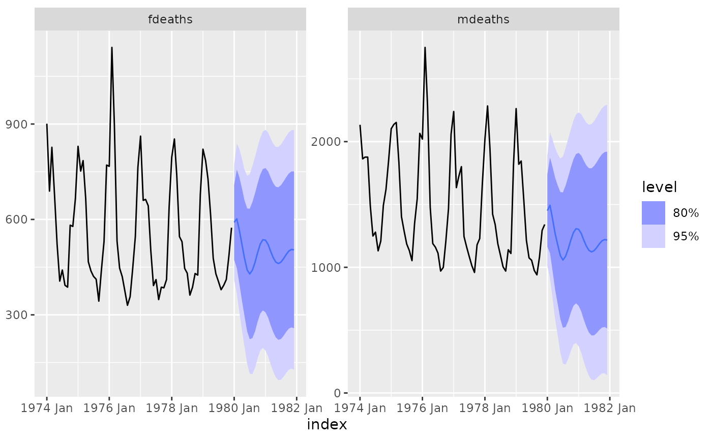
  autoplot(lung_deaths)